Simulating Langevin Equation for Brownian Motion
Here, we are going to look at how to simulate the dynamics of a Brownian particle. I will use Python programming language for the demonstration. However, readers are encouraged to use any program they find suitable. Let's start with the Langevin equation to be solved. Restricting ourself to one dimension, we have, $$ m \frac{d^2 x}{dt^2} = -\gamma v(t) + \sqrt{2 \gamma k_BT}\ \eta(t) $$ Here, the "White noise" $\eta(t)$ has the properties $$ \langle \eta(t) \rangle = 0 \ \ \ \text{and}\ \ \ \ \langle \eta(t) \eta(t') \rangle = \delta(t - t') $$ The above equation can be rewritten as $$ dv = -\frac{\gamma}{m} v dt + \sqrt{2 \gamma k_BT}\ \eta dt $$ The third term in the RHS can be identified as the differential of Wiener process: $$ dW = \eta dt $$ Since the process $W$ has Gaussian increments, we have, $$ dW = W(t + dt) - W(dt) \sim \sqrt{dt}\ \mathcal{N}(0, 1) $$ where $\mathcal{N}(0,1)$ denotes standard normal distribution. The Brownian motion, then can be simulated using Euler Maruyama Method. For the purpose of numerical simulation, we will set $k_B = 1$. Now, the difference equation corresponds to above differential equation can be written as $$ v_{i + 1} = v_{i} - \frac{\gamma}{m} v_i dt + \sqrt{2 \gamma T}\ dW_i $$ A sample program for simulating trajectories of Brownian particle is given below:
import numpy as np
import matplotlib.pyplot as plt
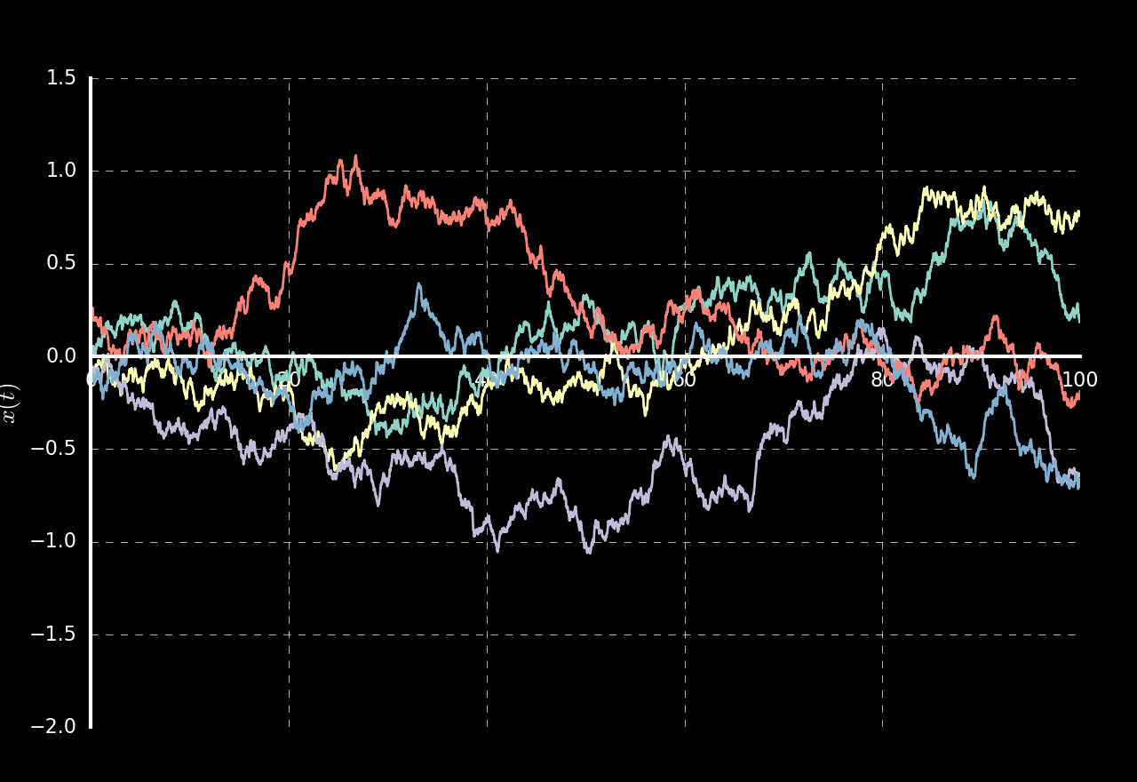
nsim = 5 # Number of simulations
Tmax = 100 # Total simulation time
dt = 0.001 # timestep
time = np.arange(0, Tmax, dt)
gamma = 5.0 # friction constant
m = 0.1 # mass of particle
T = 2.0 # Temperature
# Initial velocity is sampled from equilibrium distribution
v = np.zeros((len(time), nsim), dtype=np.float64)
v[0,:] = np.sqrt(T/m)*np.random.normal(size=nsim)
# Initial position is at origin
x = np.zeros((len(time), nsim), dtype=np.float64)
# Start of simulation
for i in range(1, len(time)):
# Velocity update
v[i, :] = v[i-1, :] - gamma/m*v[i-1, :]*dt + np.sqrt(2*gamma*T*dt)*np.random.normal(size=nsim)
# Position update
x[i, :] = x[i-1, :] + v[i, :]*dt
# Plotting
plt.style.use('dark_background')
fig = plt.figure()
ax = fig.add_subplot(1, 1, 1)
ax.spines['left'].set_position(('data',0))
ax.spines['bottom'].set_position(('data', 0))
ax.spines['right'].set_color('none')
ax.spines['top'].set_color('none')
ax.set_ylim((-2, 1.5))
ax.set_ylabel("$x(t)$", fontsize=20)
plt.plot(time, x)
plt.show()